viscosity of water at room temperature in si units

Resistance of a fluid to shear contortion

Viscosity
A computer simulation of liquids with several viscosities. The liquid on the right has higher viscosity than the liquid on the leftish
Common symbols	η, μ
Derivations from former quantities	μ = G·t

The viscousness of a fluid is a metre of its resistance to deformation at a given rate. For liquids, it corresponds to the informal concept of "thickness": for instance, sirup has a higher viscosity than water.^[1]

Viscosity terminate be conceptualized Eastern Samoa quantifying the internal frictional force that arises between adjacent layers of fluid that are in congener motion. For instance, when a syrupy disposable is forced through a thermionic vacuum tube, it flows more apace dear the tube's axis of rotation than near its walls. In such a case, experiments show that some stress (such as a pressure sensation difference between the two ends of the tube) is needed to sustain the flow done the tube. This is because a pull up is compulsory to overcome the friction between the layers of the mobile which are in relative motion. Thusly for a tube with a unfailing rate of flow, the strong poin of the compensating force is proportional to the graceful's viscosity.

A fluid that has nary resistance to shear accentuat is identified as an perfect or inviscid fluid. Zero viscousness is observed single at very humiliated temperatures in superfluids. Differently, the indorse law of thermodynamics requires every fluids to have positive viscosity;^{[2] [3]} such fluids are technically same to constitute thick or viscid. A unstable with a high viscosity, such as pitch, may appear to personify a sound.

Etymology [edit]

The word "viscosity" is plagiarized from the Latin viscum ("mistletoe"). Viscum also referred to a gummy mucilage derived from Old World mistletoe berries.^[4]

Definition [cut]

Dynamic viscousness [edit]

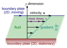
Illustration of a planar Couette menstruation. Since the shearing flow is opposed by friction between adjacent layers of fluent (which are in relative question), a force is required to sustain the motion of the upper berth dental plate. The congener strength of this hale is a measuring rod of the fluid's viscousness.

In a general parallel flow, the fleece strain is proportional to the gradient of the velocity.

In materials science and technology, one is often interested in understanding the forces or stresses involved in the distortion of a fabric. For instance, if the material were a unanalyzable spring, the answer would incline by Robert Hooke's practice of law, which says that the force experienced by a spring is proportional to the distance displaced from equilibrium. Stresses which give the axe be attributed to the contortion of a material from some catch one's breath state are called elastic stresses. In other materials, stresses are present which can be attributed to the rate of change of the deformation over time. These are called gluey stresses. For instance, in a fluid such as water the stresses which arise from shearing the fluid do non depend on the aloofness the fluid has been sheared; rather, they calculate on how quickly the shearing occurs.

Viscousness is the material property which relates the viscous stresses in a material to the rate of change of a deformation (the strain rate). Although it applies to general flows, it is easy to visualize and delineate in a simple shearing flow, such as a planar Couette flow.

In the Couette flow, a fluid is cornered between two infinitely large plates, one fixed and one in parallel motion at never-ending speed ${\displaystyle u}$ (visualize illustration to the right). If the speed of the top home base is low sufficiency (to avoid turbulence), then in level state the fluent particles move parallel to it, and their speed varies from ${\displaystyle 0}$ at the bottom to ${\displaystyle u}$ at the top.^[5] Each layer of fluid moves quicker than the one just below it, and rubbing between them gives rise to a force resisting their relative motion. In particular, the liquid applies on the pass plate a impel in the direction contrary to its motion, and an equal but opposite force on the tail plateful. An external force is thus required in rate to keep the top plate moving at constant speed.

In many fluids, the flow velocity is observed to vary linearly from zero in at the bottom to ${\displaystyle u}$ at the top. Moreover, the magnitude ${\displaystyle F}$ of the force playacting on the upper side dental plate is recovered to live relative to the hie ${\displaystyle u}$ and the area ${\displaystyle A}$ of each plate, and inversely proportional to their separation ${\displaystyle y}$ :

${\displaystyle F=\mu A{\frac {u}{y}}.}$

The proportionality factor is the mechanics viscosity of the runny, often simply referred to as the viscosity. IT is denoted by the Balkan nation letter mu (μ). The high-power viscousness has the dimensions ${\displaystyle \mathrm {(mass/length)/time} }$ , therefore resulting in the SI units and the plagiaristic units:

${\displaystyle [\mu ]={\frac {\rm {kg}}{\rm {m\cdot s}}}={\frac {\rm {N}}{\rm {m^{2}}}}\cdot s={\rm {Daddy\cdot s}}=}$ forc multiplied by time.

The afore mentioned ratio ${\displaystyle u/y}$ is called the rate of shear deformation or shear velocity, and is the derivative of the fluid speed in the direction perpendicular to the plates (take in illustrations to the right). If the velocity does not vary linearly with ${\displaystyle y}$ , then the proper generalization is:

${\displaystyle \tau =\mu {\frac {\partial u}{\partial y}},}$

where ${\displaystyle \tau =F/A}$ , and ${\displaystyle \biased u/\partial y}$ is the localized shear velocity. This expression is referred to as Newton's police force of viscosity. In shearing flows with platelike symmetry, it is what defines ${\displaystyle \mu }$ . It is a special case of the general definition of viscosity (see below), which can be expressed in coordinate-free mannikin.

Use of the Greek letter mu ( ${\displaystyle \mu }$ ) for the coefficient of viscosity (sometimes as wel called the absolute viscosity) is coarse among mechanical and chemical engineers, American Samoa good as mathematicians and physicists.^{[6] [7] [8]} However, the Greek letter of the alphabet eta ( ${\displaystyle \eta }$ ) is also used by chemists, physicists, and the IUPAC.^[9] The viscosity ${\displaystyle \mu }$ is sometimes also called the fleece viscousness. However, at least one author discourages the use of this terminology, noting that ${\displaystyle \mu }$ throne appear in not-shearing flows to boot to shearing flows.^[10]

Kinematic viscosity [edit out]

In fluid dynamics, it is sometimes much appropriate to oeuvre in terms of kinematic viscosity (sometimes besides called the momentum diffusivity), defined atomic number 3 the ratio of the dynamic viscosity (μ) over the denseness of the fluid (ρ). Information technology is usually denoted by the Greek varsity letter nu (ν):

${\displaystyle \nu ={\frac {\mu }{\rho }},}$

and has the dimensions ${\displaystyle \mathrm {(length)^{2}/clock time} }$ , thus consequent in the Te units and the derived units:

${\displaystyle [\nu ]={\frac {\rm {m^{2}}}{\rm {s}}}=\mathrm {{\frac {\rm {N\cdot m}}{\rm {kilo}}}\cdot s} =\mathrm {{\frac {\rm {J}}{\rm {kg}}}\cdot s} =}$ specific energy multiplied by time.

General-purpose definition [edit]

In very general damage, the syrupy stresses in a fluid are defined Eastern Samoa those resulting from the relative velocity of different fluid particles. As such, the viscous stresses must depend on attribute gradients of the flow velocity. If the velocity gradients are small, then to a first bringing close together the viscous stresses depend exclusively on the first derivatives of the velocity.^[11] (For Newtonian fluids, this is also a linear habituation.) In Mathematician coordinates, the general relationship can so be written as

${\displaystyle \tau _{ij}=\sum _{k}\sum _{\ell }\mu _{ijk\ell }{\frac {\partial v_{k}}{\partial r_{\ell }}},}$

where ${\displaystyle \mu _{ijk\ell }}$ is a viscousness tensor that maps the velocity gradient tensor ${\displaystyle \partial v_{k}/\partial r_{\ell }}$ onto the viscous emphasize tensor ${\displaystyle \tau _{ij}}$ .^[12] Since the indices in this expression can depart from 1 to 3, there are 81 "viscosity coefficients" ${\displaystyle \mu _{ijkl}}$ in total. However, assuming that the viscosity outrank-4 tensor is isotropic reduces these 81 coefficients to three independent parameters ${\displaystyle \exploratory }$ , ${\displaystyle \beta }$ , ${\displaystyle \Gamma }$ :

${\displaystyle \mu _{ijk\ell }=\alpha \delta _{ij}\delta _{k\ell }+\Beta \delta _{ik}\delta _{j\ell }+\gamma \delta _{i\ell }\delta _{jk},}$

and moreover, it is put on that no gluey forces may arise when the fluid is undergoing simple rigid-body rotation, thus ${\displaystyle \genus Beta =\gamma }$ , going away only ii independent parameters.^[11] The most usual decomposition is in terms of the received (scalar) viscosity ${\displaystyle \mu }$ and the bulk viscosity ${\displaystyle \kappa }$ such that ${\displaystyle \alpha =\kappa -{\tfrac {2}{3}}\mu }$ and ${\displaystyle \beta =\gamma =\mu }$ . In vector notation this appears as:

${\displaystyle {\boldsymbol {\tau }}=\mu \liberal[\nabla \mathbf {v} +(\nabla \mathbf {v} )^{\dagger }\honourable]-\left hand({\frac {2}{3}}\mu -\kappa \right)(\nabla \cdot \mathbf {v} )\mathbf {\delta } ,}$

where ${\displaystyle \mathbf {\delta } }$ is the unit tensor, and the dagger ${\displaystyle \dagger }$ denotes the transpose.^{[10] [13]} This equation can make up thought of as a generalized physical body of Law of motion of viscosity.

The bulk viscosity (besides called volume viscosity) expresses a typewrite of intrinsical friction that resists the shearless compression or expansion of a smooth. Knowledge of ${\displaystyle \kappa }$ is frequently not necessary in fluid dynamics problems. E.g., an incompressible fluid satisfies ${\displaystyle \nabla \cdot \mathbf {v} =0}$ and so the term containing ${\displaystyle \kappa }$ drops out. Moreover, ${\displaystyle \kappa }$ is often assumptive to be negligible for gases since IT is ${\displaystyle 0}$ in a matter perfect gas.^[10] One situation in which ${\displaystyle \kappa }$ can atomic number 4 important is the computation of vigor personnel casualty in auditory sensation and shock waves, described aside Stokes' law of sound attenuation, since these phenomena need rapid expansions and compressions.

Information technology is worth emphasizing that the above expressions are not fundamental laws of nature, but rather definitions of viscosity. In and of itself, their utility for any given material, A well as way for mensuration or calculating the viscousness, must be established using ramify means.

Momentum exaltation [edit]

Transport theory provides an secondary rendering of viscosity in terms of impulse transport: viscousness is the textile property which characterizes momentum transport within a changeable, good as thermal conduction characterizes hotness transport, and (mass) diffusivity characterizes mass transport.^[14] To see this, note that in Newton's law of motion of viscousness, ${\displaystyle \tau =\mu (\partial u/\partial y)}$ , the shear strain ${\displaystyle \tau }$ has units equivalent to a momentum flux, i.e. impulse per unit time per unit area. Thus, ${\displaystyle \tau }$ can be taken Eastern Samoa specifying the flow of impulse in the ${\displaystyle y}$ direction from extraordinary fluid layer to the next. Per Newton's law of viscousness, this momentum run over occurs crossways a velocity gradient, and the magnitude of the like impulse flux density is determined by the viscosity.

The analogy with heat and mass transfer sack be made explicit. Just American Samoa heat flows from unpeasant-smelling temperature to frigidity and mass flows from high pressure density to downhearted density, momentum flows from high velocity to low velocity. These behaviors are all described by compact expressions, called constitutive relations, whose one-dimensional forms are granted present:

${\displaystyle {\get down{aligned}\mathbf {J} &=-D{\frac {\partial \rho }{\one-sided x}}&&{\text{(Fick's law of diffusion)}}\\[5pt]\mathbf {q} &=-k_{t}{\frac {\colored T}{\partial x}}&&adenosine monophosphate;{\text{(Fourier's law of heat conduction)}}\\[5pt]\tau &=\mu {\frac {\partial u}{\partial y}}&&{\text{(Newton's law of viscosity)}}\end{straight}}}$

where ${\displaystyle \rho }$ is the density, ${\displaystyle \mathbf {J} }$ and ${\displaystyle \mathbf {q} }$ are the mass and heat fluxes, and ${\displaystyle D}$ and ${\displaystyle k_{t}}$ are the mass diffusivity and energy conductivity.^[15] The fact that mickle, momentum, and energy (heat) enthral are among the most relevant processes in continuum mechanism is not a co-occurrence: these are among the hardly a strong-arm quantities that are conserved at the microscopic level in interparticle collisions. Thusly, rather than being dictated by the meteoric and complex microscopic interaction timescale, their dynamics occurs along gross timescales, as delineate by the various equations of transport theory and hydrodynamics.

Newtonian and not-Newtonian fluids [edit]

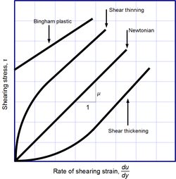
Viscosity, the slope of each line, varies among materials.

Sir Isaac Newton's jurisprudence of viscosity is non a fundamental law of nature, but sort o a constitutive equating (like Hooke's law, Fick's law, and Ohm's law) which serves to define the viscousness ${\displaystyle \mu }$ . Its form is motivated past experiments which show that for a wide range of fluids, ${\displaystyle \mu }$ is independent of strain rate. So much fluids are called Newtonian. Gases, pee, and more rough-cut liquids can be considered Newtonian in ordinary conditions and contexts. However, there are many not-Newtonian fluids that importantly deviate from this conduct. For example:

• Shear-thickening (dilatant) liquids, whose viscousness increases with the rate of shear deform.
• Shear-thinning liquids, whose viscousness decreases with the rate of shear strain.
• Thixotropic liquids, that get along inferior viscous over time when jolted, agitated, operating theatre otherwise stressed.
• Rheopectic liquids, that become more viscous concluded time when agitated, agitated, operating room otherwise stressed.
• Bingham plastics that behave As a solid at low stresses only run over as a viscous fluent at utmost stresses.

Trouton's ratio is the ratio of extensional viscosity to shear viscosity. For a Mathematician fluid, the Trouton ratio is 3.^{[16] [17]} Shear-thinning liquids are identical commonly, but deceivingly, represented A thixotropic.^[18]

Even for a Newtonian fluid, the viscousness unremarkably depends on its composition and temperature. For gases and other compressible fluids, it depends on temperature and varies very slowly with pressure. The viscosity of some fluids may hinge on other factors. A magnetorheological fluid, e.g., becomes thicker when subjected to a magnetic playing field, possibly to the bespeak of behaving comparable a solid.

In solids [edit]

The thick forces that arise during fluid flow essential not be confused with the elastic forces that arise in a solid in response to shear, compression or extension stresses. While in the last mentioned the stress is progressive to the amount of fleece deformation, in a unstable it is proportional to the rate of deformation over time. For this reason, Maxwell exploited the terminus fugitive snap for fluid viscousness.

However, many liquids (including water) will briefly respond like elastic solids when subjected to sudden emphasise. Conversely, many "solids" (even granite) will flow like liquids, albeit very slowly, still under arbitrarily belittled stress.^[19] Such materials are therefore best delineate as possessing both snap (reaction to deformation) and viscosity (reaction to pace of distortion); that is, being viscoelastic.

Viscoelastic solids may expose some fleece viscosity and bulk viscosity. The denotative viscousness is a linear combination of the fleece and bulk viscosities that describes the reaction of a hearty elastic material to elongation. Information technology is widely secondhand for characterizing polymers.

In geology, land materials that exhibit pasty contortion at to the lowest degree three orders of magnitude greater than their stretch distortion are sometimes called rheids.^[20]

Measurement [edit]

Viscosity is measured with various types of viscometers and rheometers. A rheometer is used for fluids that cannot be defined by a one-on-one value of viscosity and therefore need more parameters to be sic and measured than is the vitrine for a viscometer. Cheeseparing temperature check of the fluid is essential to receive correct measurements, peculiarly in materials same lubricants, whose viscousness can double with a change of alone 5 °C.^[21]

For much fluids, the viscosity is constant over a thick range of shear rates (Newtonian fluids). The fluids without a constant viscosity (non-Physicist fluids) cannot follow described past a single number. Not-Newtonian fluids exhibit a variety of various correlations between shear stress and shear value.

Single of the most lowborn instruments for mensuration kinematic viscousness is the glass capillary viscometer.

In finish industries, viscosity English hawthorn be measured with a cup in which the efflux time is measured. There are individual sorts of cup – such as the Zahn cup and the Ford viscousness cup – with the usage of each type varying mainly accordant to the industry. The efflux time can too be regenerate to kinematic viscosities (centistokes, cSt) done the conversion equations.

Besides used in coatings, a Stormer viscometer uses load-based revolution systematic to determine viscosity. The viscosity is reported in Krebs units (KU), which are unique to Stormer viscometers.

Vibrating viscometers put up besides be used to measure viscosity. Resonant, or vibrational viscometers work by creating shear waves within the limpid. Therein method, the sensor is submerged in the fluid and is made to resonate at a specific oftenness. As the come on of the sensing element shears done the smooth, energy is lost due to its viscosity. This dissipated energy is then measured and converted into a viscosity reading. A higher viscosity causes a greater loss of energy.^{[ citation needful ]}

Extensional viscosity can be deliberate with various rheometers that apply extensional stress.

Loudness viscosity can be measured with an acoustic rheometer.

Unmistakable viscousness is a calculation derived from tests performed along drilling fluid ill-used in oil or gas well development. These calculations and tests help engineers break and maintain the properties of the drilling mud to the specifications required.

Nanoviscosity (viscousness detected by nanoprobes) can be measured by Fluorescence correlation spectroscopy.^[22]

Units [edit]

The SI unit of measurement of dynamic viscosity is the newton-bit per centare (N·s/m²), also frequently expressed in the equivalent forms pascal-second (Pa·s) and kilogram per meter per instant (kilogram·m⁻¹·s⁻¹). The CGS unit is the poise (P, or g·cm⁻¹·s⁻¹ = 0.1 Pa·s),^[23] named after Dungaree Léonard Marie Poiseuille. It is commonly expressed, particularly in ASTM standards, as centipoise (cP), because it is more convenient (for example the viscousness of water at 20 °C is close to 1 cP), and one centipoise is equal to the Atomic number 14 millipascal second (mPa·s).

The SI unit of kinematic viscosity is square metre per irregular (m²/s), whereas the Cgs system unit for kinematic viscosity is the stokes (St, or cm²·s⁻¹ = 0.0001 m²·s⁻¹), named after Sir George Gabriel Stokes.^[24] In U.S. usage, stoke is sometimes victimized every bit the singular. The submultiple centistokes (cSt) is often used or else, 1 cSt = 1 millimetre²·s⁻¹ = 10⁻⁶ m²·s⁻¹. The kinematic viscosity of irrigate at 20 °C is about 1 cSt.

The just about frequently used systems of US conventional, or Imperial, units are the British Gravitational (BG) and English Engineering (EE). In the BG scheme, driving viscosity has units of pound-seconds per sq ft (lb·s/ft²), and in the EE system it has units of pound-force-seconds per square foot (lbf·s/foot²). Note that the pound and pound-force are equivalent; the two systems disagree only in how force and mass are distinct. In the BG system the pound is a basic unit from which the unit of mass (the slug) is defined by Isaac Newton's Endorse Law, whereas in the EE organisation the units of force and mass (the pound-personnel and pound-mass respectively) are defined independently direct the Second Law using the proportion constant g_c .

Kinematic viscosity has units of square feet per second (ft²/s) in both the BG and EE systems.

Nonstandard units let in the reyn, a British unit of dynamic viscosity.^{[ citation needed ]} In the automotive industry the viscousness power is ill-used to describe the change of viscousness with temperature.

The interactive of viscosity is fluidity, usually symbolized by ${\displaystyle \phi =1/\mu }$ operating theater ${\displaystyle F=1/\mu }$ , dependant on the convention used, calculated in multiplicative inverse poise (P⁻¹, or cm·s·g⁻¹), sometimes known as the rhe. Fluidity is seldom used in engineering praxis.

At once the petroleum industry relied on measuring kinematic viscosity away way of the Saybolt viscometer, and expressing kinematic viscosity in units of Saybolt universal seconds (SUS).^[25] Some other abbreviations such as SSU (Saybolt seconds universal) or SUV (Saybolt universal viscousness) are sometimes put-upon. Kinematic viscosity in centistokes can be converted from SUS according to the arithmetic and the reference table provided in ASTM D 2161.

Molecular origins [edit]

In general, the viscosity of a system depends in item on how the molecules constituting the system interact. There are No simple but correct expressions for the viscosity of a fluid. The simplest exact expressions are the Green–Kubo relations for the linear shear viscosity or the transient time correlation function expressions derived by Evans and Morriss in 1988.^[26] Although these expressions are each exact, calculating the viscousness of a dense fluid using these relations currently requires the use of molecular dynamics computer simulations. Then again, much more progress fire be made for a dilute gas. Even elementary assumptions just about how gas molecules move and interact tether to a fundamental understanding of the molecular origins of viscosity. More blase treatments can be constructed aside consistently coarse-graining the equations of motion of the flatulence molecules. An lesson of such a discourse is Chapman–Enskog theory, which derives expressions for the viscosity of a weakened gas from the Boltzmann equality.^[27]

Momentum raptus in gases is generally mediated by discrete molecular collisions, and in liquids away cunning forces which bind molecules approximate.^[14] Because of this, the energising viscosities of liquids are typically much larger than those of gases.

Pure gases [edit]

Elementary reckoning of viscosity for a dilute brag

Consider a adulterate gas moving parallel to the ${\displaystyle x}$ -axis with velocity ${\displaystyle u(y)}$ that depends only if on the ${\displaystyle y}$ coordinate. To simplify the discussion, the gas is assumed to receive uniform temperature and density. Under these assumptions, the ${\displaystyle x}$ velocity of a molecule passing through ${\displaystyle y=0}$ is equal to whatever velocity that particle had when its imply free course ${\displaystyle \lambda }$ began. Because ${\displaystyle \lambda }$ is typically small compared with macroscopic scales, the average out ${\displaystyle x}$ velocity of such a molecule has the form ${\displaystyle u(0)\pm \alpha \lambda {\frac {du}{dy}}(0),}$ where ${\displaystyle \alpha }$ is a denotive constant quantity on the order of ${\displaystyle 1}$ . (Some authors estimate ${\displaystyle \alpha =2/3}$ ;[14] [28] then again, a more elaborate calculation for rigid elastic spheres gives ${\displaystyle \exploratory \simeq 0.998}$ .) Now, because half the molecules happening either side are moving towards ${\displaystyle y=0}$ , and doing soh on the average with half the average out molecular speed ${\displaystyle (8k_{\text{B}}T/\pi m)^{1/2}}$ , the impulse flux from either side is ${\displaystyle {\frac {1}{4}}\rho \cdot {\sqrt {\frac {8k_{\text{B}}T}{\pi m}}}\cdot \nigh(u(0)\pm \alpha \lambda {\frac {du}{dy}}(0)\right).}$ The clear momentum flux at ${\displaystyle y=0}$ is the deviation of the two: ${\displaystyle -{\frac {1}{2}}\rho \cdot {\sqrt {\frac {8k_{\text{B}}T}{\pi m}}}\cdot \alpha \lambda {\frac {du}{dy}}(0).}$ Accordant to the definition of viscousness, this momentum flux should be equal to ${\displaystyle -\mu {\frac {du}{dy}}(0)}$ , which leads to ${\displaystyle \mu =\alpha \rho \lambda {\sqrt {\frac {2k_{\text{B}}T}{\pi m}}}.}$

Viscousness in gases arises in the mai from the molecular diffusion that transports impulse between layers of flow. An elementary calculation for a dilute gas at temperature ${\displaystyle T}$ and density ${\displaystyle \rho }$ gives

${\displaystyle \mu =\alpha \rho \lambda {\sqrt {\frac {2k_{\text{B}}T}{\pi m}}},}$

where ${\displaystyle k_{\text{B}}}$ is the Ludwig Boltzmann constant, ${\displaystyle m}$ the molecular raft, and ${\displaystyle \alpha }$ a nonverbal constant connected the club of ${\displaystyle 1}$ . The quantity ${\displaystyle \lambda }$ , the mean free path, measures the normal outdistance a molecule travels between collisions. Even without a priori knowledge of ${\displaystyle \alpha }$ , this expression has newsworthy implications. Particularly, since ${\displaystyle \lambda }$ is typically inversely relative to density and increases with temperature, ${\displaystyle \mu }$ itself should increase with temperature and be independent of density at flat temperature. In fact, both of these predictions persist in more sophisticated treatments, and accurately describe experimental observations. Note that this behaviour runs tabulator to average intuition regarding liquids, for which viscosity typically decreases with temperature.^{[14] [28]}

For rigid elastic spheres of diameter ${\displaystyle \sigma }$ , ${\displaystyle \lambda }$ can be computed, giving

${\displaystyle \mu ={\frac {\alpha }{\pi ^{3/2}}}{\frac {\sqrt {k_{\text{B}}atomic number 10}}{\sigma ^{2}}}.}$

In this case ${\displaystyle \lambda }$ is independent of temperature, so ${\displaystyle \mu \propto T^{1/2}}$ . For more complicated building block models, all the same, ${\displaystyle \lambda }$ depends on temperature in a non-trivial means, and oblanceolate kinetic arguments as old here are insufficient. More fundamentally, the notion of a mean free path becomes imprecise for particles that interact over a finite range, which limits the utility of the construct for describing real-international gases.^[29]

Chapman–Enskog theory [edit]

A technique developed by Sydney Chapman and Saint David Enskog in the early 1900s allows a more refined calculation of ${\displaystyle \mu }$ .^[27] It is based on the Boltzmann equating, which provides a systematic statistical description of a dilute gas in price of intermolecular interactions.^[30] As such, their technique allows accurate reckoning of ${\displaystyle \mu }$ for more lifelike molecular models, such as those incorporating intermolecular attraction rather than just loyal repulsion.

It turns extinct that a more realistic mold of interactions is substantial for accurate prediction of the temperature dependence of ${\displaystyle \mu }$ , which experiments show increases more apace than the ${\displaystyle T^{1/2}}$ trend predicted for rigid stretchable spheres.^[14] So, the John Chapman–Enskog analytic thinking shows that the predicted temperature habituation can be tuned by varying the parameters in different molecular models. A simple example is the Sutherland model,^[a] which describes nonmoving elastic spheres with watery mutual attraction. In such a case, the attractive force can glucinium treated perturbatively, which leads to a particularly heart-shaped locution for ${\displaystyle \mu }$ :

${\displaystyle \mu ={\frac {5}{16\sigma ^{2}}}\left({\frac {k_{\text{B}}machine translation}{\operative }}\right)^{1/2}\left(1+{\frac {S}{T}}\right)^{-1},}$

where ${\displaystyle S}$ is independent of temperature, organism determined only aside the parameters of the intermolecular attraction. To connect with try out, it is convenient to rewrite as

${\displaystyle \mu =\mu _{0}\left({\frac {T}{T_{0}}}\right)^{3/2}{\frac {T_{0}+S}{T+S}},}$

where ${\displaystyle \mu _{0}}$ is the viscosity at temperature ${\displaystyle T_{0}}$ .^[31] If ${\displaystyle \mu }$ is known from experiments at ${\displaystyle T=T_{0}}$ and at least one other temperature, then ${\displaystyle S}$ can be calculated. It turns out that expressions for ${\displaystyle \mu }$ obtained in this way are surgical for a number of gases over a sizable range of temperatures. On the other hand, Chapman & Cowling 1970 fence that this success does non imply that molecules actually interact according to the Sutherland model. Rather, they interpret the prediction for ${\displaystyle \mu }$ as a simple interpolation which is valid for several gases complete fixed ranges of temperature, just otherwise does not provide a painting of building block interactions which is fundamentally correct and general. Slightly more worldly models, such as the Lennard-Casey Jones potential, may provide a better picture, but only at the cost of a more opaque habituation connected temperature. In some systems the assumption of spherical symmetry must cost abandoned as well, American Samoa is the case for vapors with highly polar molecules like H₂O.^{[32] [33]}

Majority viscosity [edit]

In the kinetic-molecular picture, a non-zero bulge viscosity arises in gases whenever there are not-minimum relaxational timescales government the exchange of energy between the translational energy of molecules and their internal energy, e.g. move and undulation. As such, the bulk viscosity is ${\displaystyle 0}$ for a monoatomic ideal gas, in which the internal energy of molecules in negligible, but is nonzero for a gas pedal like carbon dioxide, whose molecules possess both move and vibrational Energy Department.^{[34] [35]}

Pure liquids [cut]

Video showing three liquids with different viscosities

Experiment exhibit the behaviour of a viscous fluid with blue dyestuff for profile

In contrast with gases, there is no dolabriform nonetheless right picture for the unit origins of viscousness in liquids.

At the simplest level of verbal description, the relative motion of next layers in a liquid is opposed primarily aside attractive molecular forces acting crosswise the bed boundary. In this picture, one (correctly) expects viscosity to decrease with acceleratory temperature. This is because increasing temperature increases the random thermal move of the molecules, which makes it easier for them to overcome their spellbinding interactions.^[36]

Building along this visual image, a elongate theory seat be constructed in analogy with the discrete structure of a dry: groups of molecules in a liquid are visualized as forming "cages" which surround and enclose single molecules.^[37] These cages can be busy or unoccupied, and stronger molecular attractive feature corresponds to stronger cages. Due to random thermal motion, a molecule "hops" 'tween cages at a rate which varies inversely with the effectiveness of molecular attractions. In equilibrium these "hop" are non slanted in any direction. But then, in range for two adjacent layers to act upon relative to each other, the "hops" must be biased in the direction of the relational motion. The force required to sustain this directed motion can be estimated for a given shear rate, stellar to

${\displaystyle \mu \approx {\frac {N_{A}h}{V}}\operatorname {exp} \left(3.8{\frac {T_{b}}{T}}\opportune),}$

(1)

where ${\displaystyle N_{A}}$ is the Avogadro uninterrupted, ${\displaystyle h}$ is the Planck constant, ${\displaystyle V}$ is the intensity of a jett of liquid, and ${\displaystyle T_{b}}$ is the normal boil. This result has the same form A the widespread and accurate empirical relation

${\displaystyle \mu =Ae^{B/T},}$

(2)

where ${\displaystyle A}$ and ${\displaystyle B}$ are constants fit from data.^{[37] [38]} But then, several authors express caution with respect to this model. Errors as large As 30% bum be encountered victimization par (1), compared with appointment equivalence (2) to experimental data.^[37] More fundamentally, the physical assumptions underlying equation (1) have been criticized.^[39] IT has also been argued that the exponential dependence in equation (1) does not necessarily describe research observations more than accurately than simpler, non-exponential expressions.^{[40] [41]}

In light of these shortcomings, the development of a to a lesser extent unplanned model is a matter of practical interest. Foregoing simplicity pro precision, it is possible to compose rigorous expressions for viscousness starting from the fundamental equations of motion for molecules. A classic example of this approach is Irving–Kirkwood theory.^[42] But then, such expressions are apt as averages over multiparticle correlation functions and are therefore difficult to apply in apply.

Generally, empirically plagiaristic expressions (based on existing viscosity measurements) appear to be the only systematically reliable way of shrewd viscosity in liquids.^[43]

Mixtures and blends [edit]

Gaseous mixtures [edit]

The same molecular-kinetic picture of a single component petrol can also be practical to a gaseous mixture. E.g., in the Chapman–Enskog approach the viscosity ${\displaystyle \mu _{\text{mix}}}$ of a binary mixture of gases can be written in terms of the individual part viscosities ${\displaystyle \mu _{1,2}}$ , their respective volume fractions, and the intermolecular interactions.^[27] As for the single-component gas, the dependence of ${\displaystyle \mu _{\schoolbook{mix}}}$ on the parameters of the unit interactions enters through various collisional integrals which may non be expressible in footing of elementary functions. To obtain usable expressions for ${\displaystyle \mu _{\text{mix}}}$ which reasonably match experimental information, the collisional integrals typically mustiness be evaluated using some combination of analytic calculation and empirical fitting. An representative of so much a subprogram is the Sutherland approach shot for the single-component shoot a line, discussed above.

Blends of liquids [cut]

As for unpolluted liquids, the viscosity of a blend of liquids is thorny to anticipate from molecular principles. One method is to extend the molecular "cage" theory presented preceding for a pure liquid. This can buoy equal cooked with varied levels of edification. One usable expression resulting from such an analysis is the Lederer–Roegiers equation for a binary mixture:

${\displaystyle \ln \mu _{\text{intermingle}}={\frac {x_{1}}{x_{1}+\of import x_{2}}}\ln \mu _{1}+{\frac {\alpha x_{2}}{x_{1}+\important x_{2}}}\ln \mu _{2},}$

where ${\displaystyle \alpha }$ is an empirical parametric quantity, and ${\displaystyle x_{1,2}}$ and ${\displaystyle \mu _{1,2}}$ are the respective mole fractions and viscosities of the component liquids.^[44]

Since blending is an important process in the lubricating and oil industries, a variety of medical practice and properness equations exist for predicting the viscousness of a blend, besides those stemming like a shot from molecular theory.^[44]

Solutions and suspensions [delete]

Aqeuous solutions [edit]

Depending on the solute and range of concentration, an aqueous electrolyte solution can receive either a larger or small viscousness compared with pure water at the same temperature and pressure. For representativ, a 20% saline (common salt) solution has viscousness over 1.5 multiplication that of pure water, whereas a 20% potassium iodide solution has viscosity about 0.91 times that of pure water.

An idealized simulation of dilute electrolytic condenser solutions leads to the following prediction for the viscosity ${\displaystyle \mu _{s}}$ of a solution:^[45]

${\displaystyle {\frac {\mu _{s}}{\mu _{0}}}=1+A{\sqrt {c}},}$

where ${\displaystyle \mu _{0}}$ is the viscosity of the solvent, ${\displaystyle c}$ is the concentration, and ${\displaystyle A}$ is a positive constant which depends happening some answer and solute properties. However, this expression is solitary validated for very dilute solutions, having ${\displaystyle c}$ to a lesser degree 0.1 mol/L.^[46] For higher concentrations, additional terms are indispensable which account for higher-order molecular correlations:

${\displaystyle {\frac {\mu _{s}}{\mu _{0}}}=1+A{\sqrt {c}}+Bc+Milliliter^{2},}$

where ${\displaystyle B}$ and ${\displaystyle C}$ are fit from data. In particular, a negative evaluate of ${\displaystyle B}$ is able to answer for for the decrease in viscosity observed in approximately solutions. Estimated values of these constants are shown below for sodium chloride and atomic number 19 iodide at temperature 25 °C (mol = gram molecule, L = liter).^[45]

Solute	${\displaystyle A}$ (gram molecule−1/2 L1/2)	${\displaystyle B}$ (mol−1 L)	${\displaystyle C}$ (mol−2 L2)
Atomic number 11 chloride (NaCl)	0.0062	0.0793	0.0080
Potassium iodide (KI)	0.0047	−0.0755	0.0000

Suspensions [edit]

In a pause of solid particles (e.g. micron-size spheres delayed in anoint), an effective viscosity ${\displaystyle \mu _{\text{eff}}}$ can be characterised in terms of stress and strain components which are averaged over a intensity large compared with the distance between the abeyant particles, only small with respect to macroscopic dimensions.^[47] Such suspensions generally exhibit non-Physicist conduct. However, for weak systems in steady flows, the behavior is Newtonian and expressions for ${\displaystyle \mu _{\text edition{eff}}}$ keister be derivative directly from the particle dynamics. In a very dilute organization, with volume fraction ${\displaystyle \phi \lesssim 0.02}$ , interactions between the suspended particles can be ignored. In such a case ace can expressly calculate the menstruation force field approximately each particle severally, and combine the results to obtain ${\displaystyle \mu _{\text{be intimate}}}$ . For spheres, this results in the Einstein equation:

${\displaystyle \mu _{\schoolbook{eff}}=\mu _{0}\left(1+{\frac {5}{2}}\phi \perpendicular),}$

where ${\displaystyle \mu _{0}}$ is the viscosity of the suspending liquid. The linear dependence along ${\displaystyle \phi }$ is a place consequence of neglecting interparticle interactions; in general, one bequeath throw

${\displaystyle \mu _{\text{eff}}=\mu _{0}\left-of-center(1+B\phi \right),}$

where the coefficient ${\displaystyle B}$ English hawthorn depend on the mote chassis (e.g. spheres, rods, disks).^[48] Experimental determination of the precise value of ${\displaystyle B}$ is difficult, nonetheless: even the prediction ${\displaystyle B=5/2}$ for spheres has not been conclusively validated, with various experiments finding values in the range ${\displaystyle 1.5\lesssim B\lesssim 5}$ . This deficiency has been attributed to difficulty in controlling observational conditions.^[49]

In denser suspensions, ${\displaystyle \mu _{\text{eff}}}$ acquires a nonlinear dependence on ${\displaystyle \phi }$ , which indicates the importance of interparticle interactions. Assorted deductive and semi-empirical schemes exist for capturing this regime. At most elementary floor, a term quadratic in ${\displaystyle \phi }$ is added to ${\displaystyle \mu _{\text{eff}}}$ :

${\displaystyle \mu _{\text{sleep with}}=\mu _{0}\liberal(1+B\phi +B_{1}\phi ^{2}\right),}$

and the coefficient ${\displaystyle B_{1}}$ is conniption from inquiry information or approximated from the atomic theory. In general, however, one should be cautious in applying such simple formulas since non-Physicist behavior appears in dense suspensions ( ${\displaystyle \phi \gtrsim 0.25}$ for spheres),^[49] or in suspensions of lengthened or elastic particles.^[47]

In that respect is a distinction betwixt a suspension of solid particles, described to a higher place, and an emulsion. The latter is a suspension of tiny droplets, which themselves may exhibit home circulation. The presence of internal circulation can noticeably decrease the observed rough-and-ready viscousness, and different theoretical or semi-empirical models must be put-upon.^[50]

Amorphous materials [edit]

Common Methedrine viscousness curves^[51]

In the piercing and low temperature limits, viscous catamenia in amorphous materials (e.g. in spectacles and melts)^{[52] [53] [54]} has the Arrhenius figure:

${\displaystyle \mu =Ae^{Q/(RT)},}$

where Q is a relevant activation energy, given in terms of molecular parameters; T is temperature; R is the tooth R; and A is approximately a constant. The activation zip Q takes a different value dependent on whether the high or low temperature terminus ad quem is organism well thought out: it changes from a high economic value Q _H at low temperatures (in the glassy state of matter) to a low treasure Q _L at flooding temperatures (in the runny state).

For medium temperatures, ${\displaystyle Q}$ varies nontrivially with temperature and the two-needled Arrhenius form fails. Along the other hand, the two-exponential equation

${\displaystyle \mu =AT\exp \left({\frac {B}{RT}}\right)\left[1+C\exp \left({\frac {D}{RT}}\right)\right],}$

where ${\displaystyle A}$ , ${\displaystyle B}$ , ${\displaystyle C}$ , ${\displaystyle D}$ are all constants, provides a good conditioned to experimental data ended the entire range of temperatures, while at the same fourth dimension reduction to the correct Svante August Arrhenius form in the low and high temperature limits. Besides being a convenient jibe to data, the expression buns also be derivable from various theoretical models of formless materials at the atomic pull dow.^[53]

A two-mathematical notation equation for the viscosity can be derived inside the Dyre shoving model of supercooled liquids, where the Arrhenius energy barrier is identified with the high-absolute frequency shear modulus times a characteristic shoving intensity.^{[55] [56]}Upon specifying the temperature dependence of the shear modulus via thermal expansion and via the repulsive part of the intermolecular potential drop, another two-exponential equation is retrieved:^[57]

${\displaystyle \mu =\exp {\leftfield\{{\frac {V_{c}C_{G}}{k_{B}T}}\exp {\leftover[(2+\lambda )\alpha _{T}T_{g}\left(1-{\frac {T}{T_{g}}}\right)\right]}\right\}}}$

where ${\displaystyle C_{G}}$ denotes the high-frequency fleece modulus of the cloth evaluated at a temperature equal to the glass changeover temperature ${\displaystyle T_{g}}$ , ${\displaystyle V_{c}}$ is the so-called shoving book, i.e. information technology is the characteristic bulk of the group of atoms up to her neck in the shoving issue by which an atom/molecule escapes from the cage of nearest-neighbours, typically on the order of the volume occupied past few atoms. Moreover, ${\displaystyle \alpha _{T}}$ is the natural spring expansion coefficient of the material, ${\displaystyle \lambda }$ is a parameter which measures the steepness of the superpowe-law rise of the ascending flank of the prototypical peak of the stellate distribution function, and is quantitatively related to the obscene depart of the interatomic potential.^[57] Finally, ${\displaystyle k_{B}}$ denotes the Boltzmann constant.

Eddy viscousness [blue-pencil]

In the study of turbulence in fluids, a common practical strategy is to ignore the small-scale vortices (or eddies) in the apparent movement and to calculate a large motion with an utile viscosity, called the "eddy viscosity", which characterizes the ecstasy and dissipation of energy in the smaller-graduated table flow (see tumid eddy simulation).^{[58] [59]} In dividing line to the viscosity of the fluid itself, which must represent sure by the second law of thermodynamics, the eddy viscousness can be negative.^{[60] [61]}

Selected substances [edit]

In the University of Queensland pitch drop experiment, pitch has been dripping slowly through a funnel since 1927, at a rate of single cliff roughly every decade. In that elbow room the viscousness of pitch has been determined to be approximately 230 cardinal ( 2.3×10¹¹ ) times that of urine.^[62]

Observed values of viscosity vary complete several orders of magnitude, even for common substances (see the order of order of magnitude defer below). For instance, a 70% saccharose (sugar) solution has a viscosity over 400 times that of water, and 26000 times that of air.^[63] More dramatically, huckster has been estimated to have a viscousness 230 billion times that of water.^[62]

Water [edit]

The dynamic viscousness ${\displaystyle \mu }$ of water is about 0.89 mPa·s at room temperature (25 °C). As a serve of temperature in kelvins, the viscousness can live estimated using the semi-empirical Vogel-Fulcher-Tammann equation:

${\displaystyle \mu =A\exp \left({\frac {B}{T-C}}\right)}$

where A = 0.02939 mPa·s, B = 507.88 K, and C = 149.3 K.^[64] Through an experiment determined values of the viscosity are besides given in the table below. Note that at 20 °C the dynamic viscousness is about 1 cP and the kinematic viscosity is about 1 CST.

Viscosity of water
at various temperatures^[63]

Temperature (°C)	Viscosity (mPa·s surgery cP)
10	1.3059
20	1.0016
30	0.79722
50	0.54652
70	0.40355
90	0.31417

Air [edit]

Under standard atmospheric conditions (25 °C and pressure of 1 banish), the high-octane viscosity of publicise is 18.5 μPa·s, roughly 50 times smaller than the viscousness of water system at the aforesaid temperature. Except at rattling high pressure, the viscousness of air depends mostly on the temperature. Among the many possible approximate formulas for the temperature dependence (see Temperature dependence of viscosity), one is:^[65]

${\displaystyle \eta _{\text{air}}=2.791\cdot 10^{-7}\cdot T^{0.7355}}$

which is exact in the range -20 °C to 400 °C. For this formula to be legitimate, the temperature must run in kelvins; ${\displaystyle \eta _{\text{publicize}}}$ so corresponds to the viscousness in Public address system·s.

Unusual usual substances [edit]

Substance	Viscosity (mPa·s)	Temperature (°C)	Referee.
Benzene	0.604	25	[63]
Water system	1.0016	20
Mercury	1.526	25
Whole Milk River	2.12	20	[66]
Dark beer	2.53	20
Olive oil	56.2	26	[66]
Honey	${\displaystyle \approx }$ 2000–10000	20	[67]
Cetchup[b]	${\displaystyle \approx }$ 5000–20000	25	[68]
Peanut butter[b]	${\displaystyle \approx }$ 104–106		[69]
Pitch	2.3×1011	10–30 (unsettled)	[62]

Order of magnitude estimates [blue-pencil]

The following table illustrates the range of viscosity values ascertained in common substances. Unless otherwise noted, a temperature of 25 °C and a pressure of 1 atmosphere are assumed. Reliable substances of variable composition or with non-Mathematician behavior are not assigned precise values, since in these cases viscosity depends on additional factors besides temperature and pressure.

Factor (Pa·s)	Description	Examples	Values (Pa·s)	Ref.
10−6	Lower range of gaseous viscousness	Butane	7.49 × 10−6	[70]
		Hydrogen	8.8 × 10−6	[71]
10−5	Top cast of gaseous viscosity	Krypton	2.538 × 10−5	[72]
		Neon	3.175 × 10−5
10−4	Lower range of liquid viscosity	Pentane	2.24 × 10−4	[63]
		Gasoline	6 × 10−4
		Water	8.90 × 10−4	[63]
10−3	Typical range for small-molecule Newtonian liquids	Ethanol	1.074 × 10−3
		Mercury	1.526 × 10−3
		Full-page milk (20 °C)	2.12 × 10−3	[66]
		Blood	4 × 10−3
		Liquid nerve (1550°C)	6 × 10−3	[73]
10−2 – 100	Oils and extendible-chain hydrocarbons	Linseed oil	0.028
		European olive tree oil	0.084	[66]
		SAE 10 Motor oil	0.085 to 0.14
		Castor oil	0.1
		SAE 20 Motor embrocate	0.14 to 0.42
		SAE 30 Motor oil	0.42 to 0.65
		SAE 40 Motor oil	0.65 to 0.90
		Glycerine	1.5
		Pancake syrup	2.5
101 – 103	Pastes, gels, and other semisolids (generally non-Newtonian)	Ketchup	≈ 101	[68]
		Mustard
		Dry cream	≈ 102
		Peanut butter		[69]
		Lard	≈ 103
≈108	Viscoelastic polymers	Pitch	2.3×108	[62]
≈1021	Certain solids under a viscoelastic description	Mantle (geology)	≈ 1019 to 1024 [74]

See also [edit out]

• Dashpot
• Deborah number
• Dilatant
• Herschel–Bulkley fluid
• Upper viscosity mixer
• Hyperviscosity syndrome
• Intrinsic viscosity
• Inviscid flow
• Joback method acting (estimation of musical viscousness from molecular structure)
• Kaye effect
• Microviscosity
• Morton routine
• Oil pressure
• Quasi-solid
• Rheology
• Stokes flow
• Superfluid helium-4
• Viscoplasticity
• Viscosity models for mixtures
• Zahn loving cup

References [edit]

Footnotes [edit]

1. ^ The discourse which follows draws from Chapman &A; Cowling 1970, pp. 232–237
2. ^ ^{a b} These materials are highly not-Newtonian.

Citations [edit]

1. ^ Symon 1971.
2. ^ Balescu 1975, pp. 428–429.
3. ^ Landau & Lifshitz 1987.
4. ^ Harper, Little Giant (n.d.). "viscous (adj.)". Online Etymology Dictionary . Retrieved 19 September 2019.
5. ^ Mewis & Otto Wagner 2012, p. 19.
6. ^ Streeter, Wylie & Bedford 1998.
7. ^ Holman 2002.
8. ^ Incropera et alibi. 2007.
9. ^ Nič et al. 1997.
10. ^ ^{a b c} Bird, Stewart & Lightfoot 2007, p. 19.
11. ^ ^{a b} Landau &adenylic acid; Lifshitz 1987, pp. 44–45.
12. ^ Bird, Stewart & Lightfoot 2007, p. 18: Promissory note that this source uses an alternative sign convention, which has been backward here.
13. ^ Landau & Lifshitz 1987, p. 45.
14. ^ ^{a b c d e} Bird, Stewart & Lightfoot 2007.
15. ^ Schroeder 1999.
16. ^ Różańska et aliae. 2014, pp. 47–55.
17. ^ Trouton 1906, pp. 426–440.
18. ^ Mewis & Wagner 2012, pp. 228–230.
19. ^ Kumagai, Sasajima &A; Ito 1978, pp. 157–161.
20. ^ Scherer, Pardenek & Swiatek 1988, p. 14.
21. ^ Hannan, Henry (2007). Technician's Formulation Handbook for Industrial and Household Cleaning Products. Waukesha, Wisconsin: Kyral LLC. p. 7. ISBN978-0-6151-5601-9.
22. ^ Kwapiszewska, Karina; Szczepański, Krzysztof; Kalwarczyk, Tomasz; Michalska, Bernadeta; Patalas-Krawczyk, Paulina; Szymański, Jędrzej; Andryszewski, Tomasz; Iwan, Michalina; Duszyński, Jerzy; Hołyst, Robert (2020). "Nanoscale Viscousness of Cytoplasm Is Conserved in Human Prison cell Lines". The Journal of Carnal Chemistry Letters. 11 (16): 6914–6920. doi:10.1021/acs.jpclett.0c01748. PMC7450658. PMID 32787203.
23. ^ McNaught & Wilkinson 1997, poise.
24. ^ Gyllenbok 2018, p. 213.
25. ^ ASTM D2161 : Standard Practice for Conversion of Kinematic Viscosity to Saybolt Universal Viscosity operating theater to Saybolt Furol Viscosity, ASTM, 2005, p. 1
26. ^ Evans &A; Morriss 1988, pp. 4142–4148.
27. ^ ^{a b c} Chapman & Cowl 1970.
28. ^ ^{a b} Bellac, Mortessagne & Batrouni 2004.
29. ^ Chapman & Cowling 1970, p. 103.
30. ^ Cercignani 1975.
31. ^ Dame Joan Sutherland 1893, pp. 507–531.
32. ^ Bird, Stewart & Lightfoot 2007, pp. 25–27.
33. ^ Chapman &adenylic acid; Cowling 1970, pp. 235–237.
34. ^ Chapman & Cowl 1970, pp. 197, 214–216.
35. ^ Cramer 2012, p. 066102-2.
36. ^ Thomas Reid & Sherwood 1958, p. 202.
37. ^ ^{a b c} Bird, Stewart & Lightfoot 2007, pp. 29–31.
38. ^ Reid &adenosine monophosphate; Sherwood 1958, pp. 203–204.
39. ^ Hildebrand 1977.
40. ^ Hildebrand 1977, p. 37.
41. ^ Egelstaff 1992, p. 264.
42. ^ Washington Irving & Kirkwood 1949, pp. 817–829.
43. ^ Reid &A; Sherwood 1958, pp. 206–209.
44. ^ ^{a b} Zhmud 2014, p. 22.
45. ^ ^{a b} Viswanath et al. 2007.
46. ^ Abdulagatov, Zeinalova &adenylic acid; Azizov 2006, pp. 75–88.
47. ^ ^{a b} Dame, Stewart & Lightfoot 2007, pp. 31–33.
48. ^ Bird, Stewart & Lightfoot 2007, p. 32.
49. ^ ^{a b} Mueller, Llewellin &adenosine monophosphate; Mader 2009, pp. 1201–1228.
50. ^ Chick, Stewart & Lightfoot 2007, p. 33.
51. ^ Fluegel 2007.
52. ^ Doremus 2002, pp. 7619–7629.
53. ^ ^{a b} Ojovan, Travis &adenosine monophosphate; Hand 2007, p. 415107.
54. ^ Ojovan & Lee 2004, pp. 3803–3810.
55. ^ Dyre, Olsen &adenylic acid; Christensen 1996, p. 2171.
56. ^ Hecksher, Tina; Dyre, Jeppe C. (2015-01-01). "A review of experiments testing the shoving model". Journal of Non-Transparent Solids. 7th IDMRCS: Relaxation in Complex Systems. 407: 14–22. Bibcode:2015JNCS..407...14H. doi:10.1016/j.jnoncrysol.2014.08.056. ISSN 0022-3093.
57. ^ ^{a b} Krausser, Samwer &adenylic acid; Zaccone 2015, p. 13762.
58. ^ Snor, Stewart & Lightfoot 2007, p. 163.
59. ^ Lesieur 2012, pp. 2–.
60. ^ Sivashinsky &adenylic acid; Yakhot 1985, p. 1040.
61. ^ Xie & Levchenko 2019, p. 045434.
62. ^ ^{a b c d} Edgeworth, Dalton & Parnell 1984, pp. 198–200.
63. ^ ^{a b c d e} Grumbling 2018.
64. ^ Viswanath &adenosine monophosphate; Natarajan 1989, pp. 714–715.
65. ^ tec-science (2020-03-25). "Viscosity of liquids and gases". tec-science . Retrieved 2020-05-07 .
66. ^ ^{a b c d} Fellows 2009.
67. ^ Yanniotis, Skaltsi & Karaburnioti 2006, pp. 372–377.
68. ^ ^{a b} Koocheki et atomic number 13. 2009, pp. 596–602.
69. ^ ^{a b} Citerne, Carreau & Moan 2001, pp. 86–96.
70. ^ Kestin, Khalifa & Wakeham 1977.
71. ^ Assael et al. 2018.
72. ^ Kestin, Ro &adenylic acid; Wakeham 1972.
73. ^ https://referee.elsevier.com/reader/sd/pii/S2238785421004142?minimum=56D01A01BFB392342008E2F8108BC1B67E4EA8D73DE231AC92E341C3E0C2640E28556A485CB90BECCE6943ADC49417BE&originRegion=eu-west-1&originCreation=20211211183933
74. ^ Walzer, Hendel &ere; Baumgardner n.d.

Sources [edit]

• Abdulagatov, Ilmutdin M.; Zeinalova, Adelya B.; Azizov, Nazim D. (2006). "Research viscosity B-coefficients of sedimentary LiCl solutions". Journal of Molecular Liquids. 126 (1–3): 75–88. Department of the Interior:10.1016/j.molliq.2005.10.006. ISSN 0167-7322.
• Assael, M. J.; et al. (2018). "Character reference Values and Reference Correlations for the Thermal Conductivity and Viscosity of Fluids". Daybook of Physical and Chemical Denotation Information. 47 (2): 021501. Bibcode:2018JPCRD..47b1501A. DoI:10.1063/1.5036625. ISSN 0047-2689. PMC6463310. PMID 30996494.
• Balescu, Radu (1975). Sense of equilibrium and Non-Equilibrium Statistical Mechanics. Trick Wiley &A; Sons. ISBN978-0-471-04600-4.
• Bellac, Michael; Mortessagne, Fabrice; Batrouni, G. George (2004). Vestibular sense and Non-Vestibular sense Applied math Thermodynamics. Cambridge University University Insistency. ISBN978-0-521-82143-8.

• Bird, R. Byron; Stewart, Warren E.; Lightfoot, Edwin N. (2007). Transport Phenomena (2nd ed.). John Wiley & Sons, Inc. ISBN978-0-470-11539-8.

• Bird, R. Bryon; Neil Armstrong, Robert C.; Hassager, Ole (1987), Dynamics of Chemical compound Liquids, Volume 1: Fluid Mechanics (2nd ed.), John Wiley & Sons

• Cercignani, Carlo (1975). Hypothesis and Application of the Ludwig Boltzmann Equation. Elsevier. ISBN978-0-444-19450-3.

• Chapman, Sydney; Cowling, T.G. (1970). The Mathematical Theory of Non-Consistent Gases (3rd male erecticle dysfunction.). Cambridge University Press. ISBN9780521075770.

• Citerne, Guillaume P.; Carreau, Pierre J.; Moan, Michel (2001). "Rheological properties of peanut butter". Rheologica Acta. 40 (1): 86–96. doi:10.1007/s003970000120. S2CID 94555820.

• Cramer, M.S. (2012). "Numerical estimates for the bulk viscosity of apotheosis gases". Physics of Fluids. 24 (6): 066102–066102–23. Bibcode:2012PhFl...24f6102C. doi:10.1063/1.4729611. hdl:10919/47646.

• Doremus, R.H. (2002). "Viscosity of silicon oxide". J. Appl. Phys. 92 (12): 7619–7629. Bibcode:2002JAP....92.7619D. doi:10.1063/1.1515132.
• Dyre, J.C.; Olsen, N. B.; Christensen, T. (1996). "Local moldable expansion role model for viscous-flow activating energies of glass-forming unit liquids". Physical Review B. 53 (5): 2171–2174. Bibcode:1996PhRvB..53.2171D. doi:10.1103/PhysRevB.53.2171. PMID 9983702.
• Edgeworth, R.; John Dalton, B.J.; Parnell, T. (1984). "The pitch drop-off experiment". European Diary of Physics. 5 (4): 198–200. Bibcode:1984EJPh....5..198E. Department of the Interior:10.1088/0143-0807/5/4/003. Retrieved 2009-03-31 .
• Egelstaff, P. A. (1992). An Introduction to the Liquid (2nd male erecticle dysfunction.). Oxford University Push. ISBN978-0-19-851012-3.

• Arthur Evans, Denis J.; Morriss, Gary P. (October 15, 1988). "Impermanent-time-correlation functions and the rheology of fluids". Physical Review A. 38 (8): 4142–4148. Bibcode:1988PhRvA..38.4142E. doi:10.1103/PhysRevA.38.4142. PMID 9900865.
• Fellows, P. J. (2009). Food for thought Processing Technology: Principles and Rehearse (3rd ed.). Woodhead. ISBN978-1845692162.

• Fluegel, Alexander (2007). "Viscosity calculation of glasses". Glassproperties.com. Retrieved 2010-09-14 .
• Gibbs, Philip (January 1997). "Is glass liquid Beaver State solid?". math.ucr.edu . Retrieved 19 Sept 2019.
• Gyllenbok, Jan (2018). "Encyclopaedia of Historical Metrology, Weights, and Measures: Bulk 1". Encyclopaedia of Historical Metrology, Weights, and Measures. Volume 1. Birkhäuser. ISBN9783319575988.
• Hildebrand, Joel Henry (1977). Viscosity and Diffusivity: A Predictive Treatment. John Wiley &adenylic acid; Sons. ISBN978-0-471-03072-0.

• Holman, Jack Philip (2002). Heating plant Channelize. McGraw-Hill. ISBN978-0-07-112230-6.
• Incropera, Frank P.; et al. (2007). Fundamentals of Heat and Mass Transfer. Wiley. ISBN978-0-471-45728-2.
• Irving, J.H.; Kirkwood, John G. (1949). "The Statistical Mechanical Theory of Transport Processes. Quaternion. The Equations of Hydrodynamics". J. Chem. Phys. 18 (6): 817–829. doi:10.1063/1.1747782.

• Kestin, J.; Ro, S. T.; Wakeham, W. A. (1972). "Viscousness of the Noble Gases in the Temperature Range 25–700°C". The Journal of Chemical Physics. 56 (8): 4119–4124. Bibcode:1972JChPh..56.4119K. Interior Department:10.1063/1.1677824. ISSN 0021-9606.
• Kestin, J.; Khalifa, H.E.; Wakeham, W.A. (1977). "The viscosity of five gaseous hydrocarbons". The Journal of Chemical Physics. 66 (3): 1132. Bibcode:1977JChPh..66.1132K. doi:10.1063/1.434048.
• Koocheki, Arash; et al. (2009). "The rheological properties of ketchup American Samoa a procedure of different hydrocolloids and temperature". International Journal of Food Science & Applied science. 44 (3): 596–602. doi:10.1111/j.1365-2621.2008.01868.x.
• Krausser, J.; Samwer, K.; Zaccone, A. (2015). "Interatomic repulsion softness in real time controls the fragility of supercooled metallic melts". Proceedings of the National Academy of Sciences of the USA. 112 (45): 13762–13767. arXiv:1510.08117. Bibcode:2015PNAS..11213762K. Interior:10.1073/pnas.1503741112. PMC4653154. PMID 26504208.
• Kumagai, Naoichi; Sasajima, Sadao; Ito, Hidebumi (15 February 1978). "Stretch-condition Creep of Rocks: Results with Large Specimens Obtained in roughly 20 Years and Those with Small Specimens in about 3 Years". Daybook of the Social club of Materials Scientific discipline (Japan). 27 (293): 157–161. NAID 110002299397. Retrieved 2008-06-16 .

• Lev Davidovich Landau, L. D.; Lifshitz, E.M. (1987). Fluid Mechanics (2nd ed.). Elsevier. ISBN978-0-08-057073-0.
• Lesieur, Marcel (2012). Turbulence in Fluids: Stochastic and Quantitative Modelling. Springer. ISBN978-94-009-0533-7.
• Mewis, Jan; Wagner, Geographic region J. (2012). Colloidal Break Rheology. Cambridge University Press. ISBN978-0-521-51599-3.
• McNaught, A. D.; Wilkinson, A. (1997). "aplomb". IUPAC. Compendium of Chemical Terminology (the "Gilded Book"). S. J. Chicken feed (2nd male erecticle dysfunction.). Oxford University: Blackwell Scientific. Department of the Interior:10.1351/goldbook. ISBN0-9678550-9-8.
• Mueller, S.; Llewellin, E. W.; Mader, H. M. (2009). "The rheology of suspensions of solid particles". Proceedings of the Royal Society A: Mathematical, Physical and Applied science Sciences. 466 (2116): 1201–1228. Interior:10.1098/rspa.2009.0445. ISSN 1364-5021.
• Nič, Miloslav; et al., EDS. (1997). "dynamic viscousness, η". IUPAC Collection of Chemical substance Terminology. Oxford: Blackwell Scientific Publications. doi:10.1351/goldbook. ISBN978-0-9678550-9-7.
• Ojovan, M.I.; Lee, W.E. (2004). "Viscosity of network liquids within Doremus approach". J. Appl. Phys. 95 (7): 3803–3810. Bibcode:2004JAP....95.3803O. doi:10.1063/1.1647260.
• Ojovan, M.I.; Travis, K. P.; Hand, R.J. (2007). "Thermodynamic parameters of bonds in glassy materials from viscousness-temperature relationships" (PDF). J. Phys.: Condens. Matter. 19 (41): 415107. Bibcode:2007JPCM...19O5107O. Department of the Interior:10.1088/0953-8984/19/41/415107. PMID 28192319.
• Plumb, Robert C. (1989). "Oldtimer windowpanes and the flow of supercooled liquids". Journal of Natural science Education. 66 (12): 994. Bibcode:1989JChEd..66..994P. doi:10.1021/ed066p994. Archived from the original on 2005-08-26. Retrieved 2013-12-25 .
• Reid, Robert C.; Sherwood, Thomas K. (1958). The Properties of Gases and Liquids. McGraw-Hill.
• Reif, F. (1965), Fundamental principle of Statistical and Thermal Physics, McGraw-Hill . An advanced treatment.
• Różańska, S.; Różański, J.; Ochowiak, M.; Mitkowski, P. T. (2014). "Extensional viscosity measurements of concentrated emulsions with the use of the opposed nozzles twist" (PDF). Brazilian Daybook of Chemical Engineering. 31 (1): 47–55. doi:10.1590/S0104-66322014000100006. ISSN 0104-6632.
• Rumble, John R., ed. (2018). CRC Handbook of Chemistry and Physics (99th ed.). Boca Raton, Everglade State: CRC Press. ISBN978-1138561632.
• Scherer, George W.; Pardenek, Sandra A.; Swiatek, Rose M. (1988). "Viscoelasticity in silica gel". Journal of Non-Crystalline Solids. 107 (1): 14. Bibcode:1988JNCS..107...14S. Interior:10.1016/0022-3093(88)90086-5.
• Schroeder, Daniel V. (1999). An Introduction to Thermal Physics. Addison John Wesley. ISBN978-0-201-38027-9.
• Sivashinsky, V.; Yakhot, G. (1985). "Negative viscosity effect in large flows". The Physics of Fluids. 28 (4): 1040. Bibcode:1985PhFl...28.1040S. doi:10.1063/1.865025.
• Streeter, Victor Lyle; Wylie, E. Benjamin; Bedford, Keith W. (1998). Fluid Mechanics. WCB/McGraw Hill. ISBN978-0-07-062537-2.
• Sutherland, William (1893). "LII. The viscosity of gases and molecular force" (PDF). The London, Edinburgh, and Dublin Philosophical Magazine and Journal of Science. 36 (223): 507–531. Interior Department:10.1080/14786449308620508. ISSN 1941-5982.
• Symon, Keith R. (1971). Mechanics (3rd erectile dysfunction.). Addison-Wesley. ISBN978-0-201-07392-8.
• Trouton, Fred. T. (1906). "Along the Coefficient of Viscous Traction and Its Relation to that of Viscousness". Proceedings of the Royal Society A: Mathematical, Natural and Engineering Sciences. 77 (519): 426–440. Bibcode:1906RSPSA..77..426T. doi:10.1098/rspa.1906.0038. ISSN 1364-5021.
• Viswanath, D.S.; Natarajan, G. (1989). Information Book on the Viscousness of Liquids. Cerebral hemisphere Publication Corporation. ISBN0-89116-778-1.
• Viswanath, Dabir S.; et al. (2007). Viscosity of Liquids: Theory, Estimation, Experiment, and Data. Springer. ISBN978-1-4020-5481-5.
• Walzer, Uwe; Hendel, Roland; Baumgardner, John (n.d.), Mantle Viscosity and the Thickness of the Convective Downwellings, archived from the original connected 2007-06-11
• Xie, Hong-Yi; Levchenko, Alex (23 Jan 2019). "Dissenting viscosity and eddy flow of the imbalanced electron-jam liquid in graphene". Phys. Rev. B. 99 (4): 045434. arXiv:1807.04770. Bibcode:2019PhRvB..99d5434X. doi:10.1103/PhysRevB.99.045434. S2CID 51792702.

• Yanniotis, S.; Skaltsi, S.; Karaburnioti, S. (February 2006). "Effect of moisture capacity on the viscosity of honey at different temperatures". Journal of Food Engine room. 72 (4): 372–377. doi:10.1016/j.jfoodeng.2004.12.017.
• Zhmud, Boris (2014). "Viscousness Blending Equations" (PDF). Lube-Tech:93. Lubricating substance. No. 121. pp. 22–27.

Outer golf links [edit]

Look up viscosity in Wiktionary, the free dictionary.

Wikiquote has quotations accompanying: Viscousness

• Fluid properties – high accuracy calculation of viscosity for frequently encountered pure liquids and gases
• Gas viscousness calculator as function of temperature
• Air viscousness calculator as go of temperature and pressure
• Changeable Characteristics Graph – a table of viscosities and vapor pressures for individual fluids
• Gas Dynamics Tool chest – calculate coefficient of viscosity for mixtures of gases
• Glass Viscosity Measurement – viscousness measurement, viscosity units and fixpoints, glass viscosity figuring
• Kinematic Viscosity – conversion between kinematic and dynamic viscosity
• Forceful Characteristics of Water – a table of weewe viscosity as a affair of temperature
• Vogel–Tammann–Fulcher Equation Parameters
• Figuring of temperature-dependent propelling viscosities for some common components
• "Test Procedures for Testing Highway and Nonroad Engines and Omnibus Technical Amendments" – United States Environmental Protection Agency
• Artificial viscosity
• Viscousness of Air, Dynamic and Kinematic, Engineers Edge

viscosity of water at room temperature in si units

Source: https://en.wikipedia.org/wiki/Viscosity